Time-Independent Quantum Mechanics

The goal is to model any 1D Hamiltonian, $$\hat{H} = -\frac{\hbar^2}{2m}\frac{\partial^2}{\partial x^2} + V(\hat{x})$$ and find its eigenstates and eigenenergies, $$\hat{H}|\psi_n\rangle = \epsilon_n|\psi_n\rangle.$$ To do this, one needs to be able to represent the Hamiltonian operator as a matrix for a given computational basis, $|\phi_n\rangle$. We assume that the computational basis forms an orthonormal set. We start by inserting a resolution of identity in the eigenstate equation in terms of the computational basis

$$\sum_k \hat{H}|\phi_k\rangle\langle\phi_k|\psi_n\rangle = \epsilon_n\sum_k|\phi_k\rangle\langle\phi_k|\psi_n\rangle$$ Taking an overlap of the equation with with $|\phi_j\rangle$ $$\sum_k \langle\phi_j|\hat{H}|\phi_k\rangle\langle\phi_k|\psi_n\rangle = \epsilon_n\langle\phi_j|\psi_n\rangle$$ This gives rise to the matrix eigenvalue equation in the $|\phi_n\rangle$ basis.

A variety of basis can be chosen. The more physically relevant the basis, the more efficient the computations. However as long as the basis can be systematically increased, one should be able to find the correct eigenstates. This procedure is called “convergence.”

Basis of Position Eigenstates

As our first example, we choose to work in the position eigenbasis. Of course, the position eigenbasis forms an infinite dimensional vector space, which cannot be handled in a simple manner on the computer. We truncate the space by considering a subset of the real axis — the domain considered is $\mathbb{D} = [L_\text{min}, L_\text{max}] \subset\mathbb{R}$. However, that is not enough by itself because any domain, closed or open, would still be an infinite set.

So, we consider a finite set defined by a lower limit, $L_\text{min}$, an upper limit, $L_\text{max}$, and a grid spacing $\Delta x$. An arbitrary element of the computational basis is therefore $x_j = L_\text{min} + (j-1)\Delta x$, such that $\hat{x}|\phi_j\rangle = x_j|\phi_j\rangle$.

Next, we need to derive the matrix elements of the Hamiltonian. $$\langle\phi_j|\hat{H}|\phi_k\rangle = -\frac{\hbar^2}{2m}\left\langle\phi_j\left|\frac{\partial^2}{\partial x^2}\right|\phi_k\right\rangle + \langle\phi_j|V(\hat{x})|\phi_k\rangle$$ $$= -\frac{\hbar^2}{2m}\left\langle\phi_j\left|\frac{\partial^2}{\partial x^2}\right|\phi_k\right\rangle + V(x_k)\delta_{j,k}$$ Instead of directly calculating the matrix element of the second derivative operator, we start by exploring the action of the Hamiltonian matrix on an arbitrary wave function written in the position basis. $$H|\psi\rangle = -\frac{\hbar^2}{2m}\frac{\partial^2}{\partial x^2}|\psi\rangle + \hat{V}|\psi\rangle$$ So, we need to find how to write the second derivative of the wave function $|\psi\rangle$ as a function of the its values on the grid. Expanding the function in its Taylor series, we can show that $$\left.\frac{\partial^2}{\partial x^2}\psi(x)\right|_{x=x_n} (\Delta x)^2 = \psi(x_{n+1}) -2\psi(x_n) + \psi(x_{n-1})$$ $$-\frac{\hbar^2}{2m}\left.\frac{\partial^2}{\partial x^2}\psi(x)\right|_{x=x_n} = -\frac{\hbar^2}{2m(\Delta x)^2}\left(\psi(x_{n+1}) -2\psi(x_n) + \psi(x_{n-1})\right)$$ for $\Delta x\to 0$.

Now, we can put everything together. The matrix element of the Hamiltonian turns out to be: $$\langle\phi_j|\hat{H}|\phi_k\rangle = -\frac{\hbar^2}{2m(\Delta x)^2}\left(\delta_{j,k+1}-2\delta_{j,k}+\delta_{j,k-1}\right) + V(x_k)\delta_{j,k}$$

Below is the code which defines the tridiagonal Hamiltonian for a given potential on a position eigenstate basis given by the variable xgrid in Julia:

function get_Hamiltonian_matrix_position_space(; V, xgrid::AbstractVector{Float64}, hbar::Float64=1.0, m::Float64=1.0)
    dx = xgrid[2] - xgrid[1]
    Npoints = length(xgrid)
    H = zeros(Npoints, Npoints)
    for r = 1:Npoints, c = 1:Npoints
        if r == c
            H[r, c] = hbar^2 / (m * dx^2) + V(xgrid[r])
        elseif r == c-1 || r == c+1
            H[r, c] = -hbar^2 / (2 * m * dx^2)
        end
    end
    H
end

Harmonic Oscillator Eigenstates

Let us test the code by using a harmonic oscillator as an example. Consider the following potential:

V(x::Float64) = 0.5 * x^2

To use the potential, first we need to decide on the grid. This will of course be converged. Because this potential is symmetric, we will choose a symmetric grid with $L_\text{min}=-L_\text{max}$.

Let us take the following grid:

x = -0.5:0.1:0.5

using LinearAlgebra
H = get_Hamiltonian_matrix_position_space(; V, xgrid=x)
vals, vecs = eigen(H)

Take a look at the values that you get. Do they match what you know from basic quantum mechanics?

Probably not! On running the code, the lowest eigenvalue that I got is 3.43. Where are we going wrong then?

Notice that the Hamiltonian matrix elements that we derived in the previous section requires $\Delta x\to 0$. That is not being satisfied. However, what does “tending to 0” mean in a computational setting? To understand this, let us plot the energy of the lowest eigenstate as a function of $\Delta x$ keeping the $L_\text{min}$ and $L_\text{max}$ fixed. We are just trying to make the second derivative Taylor expansion correct. Notice that, in the convergence with $\Delta x$ figure, as $\Delta x$ decreases the value of $E_0$ seems to be hitting a constant value. This is the converged value with respect to $\Delta x$.

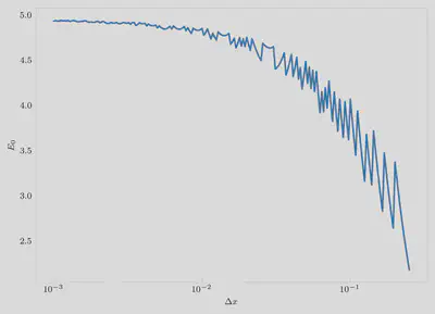
If we stopped at this level, does this value match the analytical value for the harmonic oscillator? The zero-point energy should actually be 0.5, whereas the value we are getting by diagonalizing is close to 5.0. That terribly incorrect.

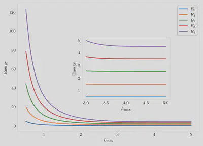
The next step would be to check for convergence with respect to the box size, $L_\text{max}$. Since the Taylor series error seems to be relatively well converged with $\Delta x=0.001$, that is kept fixed. The plot of the energies of the first five eigenstates are shown in $L_\text{max}$ convergence figure. Notice how the energies of the first 5 eigenstates converge to the correct values around $L_\text{max} = 5.0$. This is convergence with respect to the box size.

Write the programs to obtain the $\Delta x$ and the $L_\text{max}$ convergence curves.

Converge the harmonic oscillator energies corresponding to the ground state and the 10th excited state. What box-sizes are required for the two cases? Are they the same or different and why?

Can you use the same technique to converge the eigenstates of a Morse oscillator?

Basis of Momentum Eigenstates