How do we simulate the dynamics of a quantum system? Suppose we know that the initial state of the system is given by a particular wave function $|\psi(0)\rangle$ and the system is described by a Hamiltonian, $$\hat{H} = -\frac{\hbar^2}{2m}\frac{\partial^2}{\partial x^2} + V(x),$$ then the time-evolution of the wave function satisfies the Time-Dependent Schrödinger equation, $$i\hbar\frac{\partial}{\partial t}|\psi(t)\rangle = \hat{H}|\psi(t)\rangle.$$
The initial wave packet is given in position space as $\psi(x, 0)$ and we want to propagate it out to obtain $\psi(x, t)$. The direct way of solving this problem is to solve for the short-time propagator defined as $$\hat{U} = \exp\left(-\frac{i \hat{H} \Delta t}{\hbar}\right).$$ If this can be represented in position space, then we can propagate the wave function as follows: $$\psi(x, t+\Delta t) = \hat{U}\psi(x, t)$$
In the previous chapter, we have defined a function which creates the Hamiltonian in position space. We can easily exponentiate this to obtain the propagator in Julia, and use that to propagate for all times as shown below:
function propagate_accurate(H, ψ, dt, Ntimes)
    times = 0:dt:Ntimes*dt
    ψs = zeros(ComplexF64, length(ψ), length(times))
    ψs[:, 1] = ψ

    U = exp(- 1im * H * dt)

    for ts = 1:Ntimes
        ψs[:, ts+1] = U * ψs[:, ts]
    end
    times, ψs
end
Now, this works well, but the computational cost can become prohibitively high. First notice that the Hamiltonian matrix needs to be converged with respect to $L_\text{min}$, $L_\text{max}$ and $\Delta x$; one needs to use very small $\Delta x$ values to reduce the error of truncating the Taylor series for the kinetic energy part. Additionally the range has to be big enough to account for the full dynamics. Finally, the propagator is the exponential of the Hamiltonian matrix, which scales as $N^3$ where $N$ is the cardinality of the basis set. Can we do better than this?
Split-Operator Method or the Feit and Fleck Method
The propagator is the exponential of the Hamiltonian $$U(t) = \exp\left(-i \hat{H} t/\hbar\right)$$ $$=\exp\left(-i (\hat{T} + \hat{V}) t/\hbar\right)$$
The issue with directly exponentiating this operator is the computational cost. Let us see if we can simplify this expression some more. The Baker-Campbell-Hausdorff formula indicates that for any pair of operators $\hat{X}$ and $\hat{Y}$, $$\exp\left(\hat{X}\right)\exp\left(\hat{Y}\right) = \exp\left(\hat{Z}\right)$$ $$\text{where } \hat{Z} = \hat{X} + \hat{Y} + \frac{1}{2}[\hat{X}, \hat{Y}] + \frac{1}{12}[\hat{X}, [\hat{X}, \hat{Y}]] + \ldots$$
Consider the following expression: $$\exp\left(-i\hat{T}t/\hbar\right)\exp\left(-i\hat{V}t/\hbar\right) = \exp\left(-\frac{i}{\hbar}\left(\hat{H}t + \frac{1}{2}[\hat{T}, \hat{V}]t^2 + \ldots\right)\right)$$ Notice that as $t\to 0$, the right-hand side just becomes the propagator. Therefore for small $t$, the propagator can be approximated as: $$U(\Delta t) \approx \exp\left(-i \hat{T} \Delta t/\hbar\right)\exp\left(-i\hat{V}\Delta t/\hbar\right)$$ $$\approx \exp\left(-\frac{i \hat{V} \Delta t}{2\hbar}\right)\exp\left(-\frac{i \hat{T} \Delta t}{\hbar}\right)\exp\left(-\frac{i\hat{V}\Delta t}{2\hbar}\right)$$ Splitting the propagator in this manner is variously called the Suzuki-Trotter or Trotter or the Lie-Trotter decomposition. The second expression is more accurate than the first one. We will continue the discussion with the higher-order Trotter expression.
The short-time propagator needs to be applied to an initial wave function in position space. This amounts to the sequential application of individual pieces. First $\exp\left(-\frac{i\hat{V}\Delta t}{2\hbar}\right)$ needs to be applied to the wave function: $$|\psi_V\rangle = \exp\left(-\frac{i\hat{V}\Delta t}{2\hbar}\right)|\psi(t)\rangle = \int dx \exp\left(-\frac{i\hat{V}\Delta t}{2\hbar}\right)|x\rangle\langle x|\psi(t)\rangle$$ $$ = \int dx |x\rangle \underbrace{\exp\left(-\frac{iV(x)\Delta t}{2\hbar}\right)\langle x|\psi(t)\rangle}_{\psi_V(x)}$$ Next the kinetic energy portion is applied: $$\exp\left(-\frac{i\hat{T}\Delta t}{\hbar}\right)|\psi_V\rangle = \int dx_0 \exp\left(-\frac{i\hat{T}\Delta t}{\hbar}\right)|x_0\rangle \psi_V(x_0)$$ $\ket{x_0}$ is not an eigenstate of the $\hat{T}$ operator. However a momentum eigenstate, $\ket{p}$ is an eigenstate. So, we insert a resolution of identity in terms of $\ket{p}\bra{p}$ to simplify: $$\exp\left(-\frac{i\hat{T}\Delta t}{\hbar}\right)|\psi_V\rangle = \int dp\int dx_0 \exp\left(-\frac{i\hat{T}\Delta t}{\hbar}\right)\ket{p}\langle p|x_0\rangle \psi_V(x_0)$$ $$ = \frac{1}{\sqrt{2\pi\hbar}}\int dp\int dx_0 \ket{p} \exp\left(-\frac{ip^2\Delta t}{2m\hbar}\right) \exp\left(-\frac{i p x_0}{\hbar}\right) \psi_V(x_0)$$ Now, define $$\tilde{\psi}_V(p) = \frac{1}{\sqrt{2\pi\hbar}}\int dx \exp\left(-\frac{i p x}{\hbar}\right) \exp\left(-\frac{i V(x)\Delta t}{2\hbar}\right)\langle x|\psi\rangle$$ $$\therefore\ket{\psi_{TV}} = \exp\left(-\frac{i\hat{T}\Delta t}{\hbar}\right)|\psi_V\rangle = \int dp \ket{p} \underbrace{\exp\left(-\frac{ip^2\Delta t}{2m\hbar}\right) \tilde{\psi}_V(p)}_{\tilde{\psi}_{TV}(p)}$$
Finally, the last piece of the propagator in terms of the potential operator needs to be applied: $$\exp\left(-\frac{i\hat{V}\Delta t}{2\hbar}\right)\ket{\psi_{TV}} = \int dp\exp\left(-\frac{i\hat{V}\Delta t}{2\hbar}\right)\ket{p} \tilde{\psi}_{TV}(p)$$ $$= \int dx \ket{x} \int dp\exp\left(-\frac{iV(x)\Delta t}{2\hbar}\right)\langle x|p\rangle \tilde{\psi}_{TV}(p)$$ $$= \frac{1}{\sqrt{2\pi\hbar}} \int dx \ket{x} \int dp\exp\left(-\frac{iV(x)\Delta t}{2\hbar}\right)\exp\left(\frac{ipx}{\hbar}\right) \tilde{\psi}_{TV}(p)$$ $$ = \int dx \ket{x}\exp\left(-\frac{iV(x)\Delta t}{2\hbar}\right) \psi_{TV}(x)$$ where $\psi_{TV}(x) = \frac{1}{\sqrt{2\pi\hbar}}\int dp \exp(ipx/\hbar)\tilde{\psi}_{TV}(p)$.
Algorithm
Therefore, a step of propagation from $\psi(x, t)$ to $\psi(x, t+\Delta t)$ involves the following steps:
- Define $\psi_V(x) = \exp\left(-\frac{i V(x) \Delta t}{2\hbar}\right)\psi(x, t)$.
- Define $\tilde{\psi}_V(p) = \frac{1}{\sqrt{2\pi\hbar}}\int dx \exp\left(-i p x / \hbar\right)\psi_V(x)$ by using FFT.
- Apply the kinetic energy propagator $\tilde{\psi}_{TV}(p) = \exp\left(-\frac{ip^2\Delta t}{2m\hbar}\right)\tilde{\psi}_V(p)$.
- Convert to position basis: $\psi_{TV}(x) = \frac{1}{\sqrt{2\pi\hbar}}\int dp \exp\left(i p x / \hbar\right)\tilde{\psi}_{TV}(p)$ using the IFFT routines.
- Finally apply the second potential energy piece, $\psi(x, t+\Delta t) = \exp\left(-\frac{i V(x) \Delta t}{2\hbar}\right)\psi_{TV}(x)$.
Examples
Harmonic Oscillator
Imagine we are working with a harmonic potential:
V(x::Float64) = 0.5 * x^2dt = 2π/100
ntimes = 1000
ψ0 = zeros(ComplexF64, length(x))
ψ0 .= exp.(-(x .+ 3).^2 / 2.0)
ψ0 ./= sqrt(dot_product(ψ0, ψ0, dx))
times, ψs_ground = propagate_accurate(H, ψ0, dt, ntimes)function dot_product(ϕ1, ϕ2, dx)
ϕ1' * ϕ2 * dx
endThe evolution of the probability density is shown below in the gif using both
the direct exponentiation way and the split-operator method:
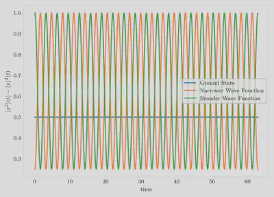
What happens if we make the initial wave packet broader or narrower than the
ground state wave packet? We keep the center of the initial wave packet at
$x=-3$ just as in the previous case.
Irrespective of the initial width of the wave function, the time evolution of
the expectation value of position is identical.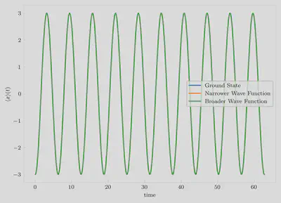
However, the widths of the wave packets show interesting patterns: