Fourier transform relates a function in one space, say the $x$ space, to another function in the reciprocal space, say the $\xi$ space.
$$F(\xi) = FT[f](\xi) = \int_{-\infty}^\infty f(x) \exp(-2\pi i\xi x) dx$$ $$f(x) = IFT[F](x) = \int_{-\infty}^\infty F(\xi) \exp(2\pi i\xi x) d\xi$$The length of the $\xi$ grid is equal to the length of the $x$ grid. Say this length is $N$. Consequently, for a particular value of $\xi$, the Fourier integral uses $N$ function evaluations. A naive calculation of the fourier transform is expensive, scaling as $\mathcal{O}(N^2)$. A much more efficient implementation is called the Fast Fourier Transform (FFT) which scales as $\mathcal{O}(N\log(N))$.
The FFTW.jl package provides implementations of FFT in Julia: $$F_k = \sum_{m=0}^{N-1} f_m \exp\left(-\frac{2\pi ikm}{N}\right)\quad k=0, \ldots, N-1.$$ This is provided by the function fft. Notice that $k$ is the discretized version of the $\xi$ variable and $m$ is the one corresponding to $x$. The points where $k>N/2$ are equivalent to frequencies at $k-N$ by periodicity. To order change this ordering to go from $-N/2$ to $N/2$, use the fftshift function provided in the FFTW.jl package. An inverse FFT routine called bfft is provided which calculates: $$f_m = \sum_{k=0}^{N-1} F_k \exp\left(\frac{2\pi ikm}{N}\right)\quad m=0, \ldots, N-1.$$
One can slowly modify the Fourier transform expression by converting it into a finite Riemann sum to obtain a formula analogous to the FFT one. Let $x$ be discretized between $x_\text{min}$ and $x_\text{max}$ in a grid of size $\Delta x$. The frequency axis will have the same $N$ number of points with a spacing of $\Delta\xi=\frac{1}{N\Delta x}$. Then the $k$th frequency component will be given as $$FT[f](k\Delta\xi) = \sum_{m=0}^{N-1} f(x_\text{min}+m\Delta x) \exp\left(-2\pi i k\Delta\xi (x_\text{min}+m\Delta x)\right)\Delta x$$ $$=\exp\left(-2\pi i k\Delta \xi x_\text{min}\right) \Delta x \sum_{m=0}^{N-1} f(x_\text{min}+m\Delta x) \exp\left(-2\pi i k\Delta \xi m \Delta x\right)$$ $$=\exp\left(-2\pi i k\Delta \xi x_\text{min}\right) \Delta x \sum_{m=0}^{N-1} f_m \exp\left(-\frac{2\pi i k m}{N}\right)$$ $$=\exp\left(-2\pi i k\Delta \xi x_\text{min}\right) \Delta x F_k$$
Now for the inverse transform: $$IFT[F](x_\text{min}+m\Delta x) = \sum_{k=0}^{N-1} F_k \exp\left(2\pi i k\Delta\xi (x_\text{min} + m\Delta x)\right)\Delta k$$ $$=\Delta k\sum_{k=0}^{N-1} \underbrace{\exp(2\pi i k\Delta\xi x_\text{min}) F_k}_{G_k} \exp\left(\frac{2\pi i k m}{N}\right)$$ $$=g_m\Delta k$$
The details of implementation in Julia are given in the examples section.
Uses in Quantum Mechanics
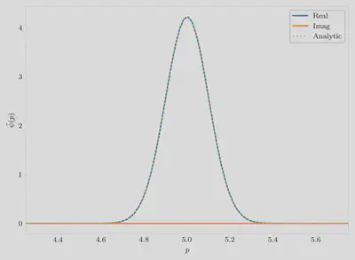
Consider a function, say the wave function, in position space, $\psi(x)$. Let us say that we want to represent that in momentum space and obtain the function $\tilde{\psi}(p)$. $$\tilde{\psi}(p) = \langle p|\psi\rangle = \int_{-\infty}^\infty dx \langle p|x\rangle\langle x|\psi\rangle$$ $$= \frac{1}{\sqrt{2\pi\hbar}}\int_{-\infty}^\infty dx \exp\left(-\frac{i p x}{\hbar}\right) \psi(x)$$ Notice that apart from the prefactor of $\frac{1}{\sqrt{2\pi\hbar}}$, the rest of the expression is a Fourier transform with the replacement $p = 2\pi\hbar\xi$. $$\tilde{\psi}(p) = \frac{1}{\sqrt{2\pi\hbar}} FT[\psi]\left(\frac{p}{2\pi\hbar}\right)$$ or, equivalently, $$\tilde{\psi}(2\pi\hbar\xi) = \frac{1}{\sqrt{2\pi\hbar}} FT[\psi]\left(\xi\right)$$
Similarly transforming the momentum space wave function back to the position space involves an inverse Fourier transform with the same definitions. $$\phi(x) = \frac{1}{\sqrt{2\pi\hbar}}\int_{-\infty}^\infty dp \exp\left(\frac{ipx}{\hbar}\right)\tilde\phi(p)$$
To prove that this works, consider transforming the momentum space wave function, obtained by Fourier transforming $\psi(x)$, back to position space: $$\psi_b(x) = \frac{1}{\sqrt{2\pi\hbar}}\int_{-\infty}^\infty \tilde\psi(p) \exp\left(\frac{ipx}{\hbar}\right) dp$$ $$=\frac{1}{2\pi\hbar} \int_{-\infty}^\infty FT[\psi]\left(\frac{p}{2\pi\hbar}\right) \exp\left(\frac{ipx}{\hbar}\right) dp$$ $$= \int_{-\infty}^\infty FT[\psi]\left(\xi\right) \exp\left(2\pi i\xi x\right) d\xi$$ $$=IFT[FT[\psi]](x) = \psi(x)$$ We get the original position space wave function back.
Example using FFTW
Let us suppose we have a wave packet that is given by: $$\psi(x) = \frac{1}{(\pi\sigma)^{1/4}} \exp\left(-\frac{x^2}{2\sigma^2} + \frac{ipx}{\hbar}\right)$$
dx = 0.01
nsteps = 2^15
x = -nsteps/2*dx:dx:nsteps/2*dx

σ = 10.0
p = 5.0
ψ = exp.(-x.^2/(2 * σ^2) + 1im * p * x) / sqrt(sqrt(π * σ))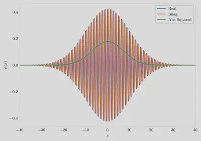
We write a function to get the Fourier transform from the FFT, keeping in mind that in almost all uses of quantum mechanics the factor of $2\pi$ in the Fourier transform kernel is absent, The inverse Fourier transform can also be implemented using FFT in a similar manner:
function inverse_fourier_transform(k, f, x, unitary::Bool=true)
    dk = k[2]-k[1]
    F = dk * bfft(ifftshift(f) .* exp.(1im * ifftshift(k) * x[1]))
    if unitary
        F ./ sqrt(2π)
    else
        F
    end
end
We use this function to obtain the momentum space wave function as follows:
k, ψtilde = fourier_transform(x, ψ)